Inference#
This guide on inference with Piscis follows the code from the run_piscis.ipynb notebook.
Step 1: Import Required Libraries
First, import the necessary libraries and Piscis modules for handling data loading, inference, and visualization.
import matplotlib.pyplot as plt
import numpy as np

from piscis import Piscis
from piscis.data import load_datasets
from piscis.downloads import download_dataset
from piscis.utils import pad_and_stack
Step 2: Download the Piscis Dataset
Download the dataset required for this example. Here, we use the dataset labeled 20251212. The download_dataset function downloads the specific dataset from our Hugging Face Dataset Repository.
download_dataset('20251212', '')
Step 3: Load the Test Dataset
Load a subset of the Piscis test dataset, pre-process the images, and extract their corresponding ground truth coordinates. The load_datasets function loads the specified dataset, and the pad_and_stack function ensures that images are padded to the same size required for model inference.
test_ds = load_datasets('20251212/A3_GFP1_A594', load_train=False, load_val=False, load_test=True)['test']
images = pad_and_stack(test_ds['x'])
coords = test_ds['y']
Note that here, only the test images and annotations are loaded, which the model never saw during training.
Step 4: Load the Piscis Model
Load the Piscis model trained using the 20251212 dataset. The Piscis class handles model weight loading and seamless scalability to large images and batches via deeptile under the hood.
model = Piscis(model_name='20251212')
When you load the model for the first time, the Piscis class will automatically call the download_pretrained_model function to download the model from our Hugging Face Model Repository.
Step 5: Run Inference on Images
Pass the test images through the model to obtain predicted coordinates and intermediate feature maps. The threshold parameter can be adjusted to filter spots based on their confidence scores.
coords_pred, y = model.predict(images, threshold=0.5, intermediates=True)
coords_pred: Predicted spot coordinates.y: Intermediate feature maps. Only returned ifintermediatesisTrue.
Step 6: Visualize Results
Visualize the input images, ground truth spots, predicted spots, and intermediate feature maps.
i = 2

fig, axs = plt.subplots(2, 3, figsize=(15, 10), sharex=True, sharey=True)

axs[0, 0].imshow(images[i])
axs[0, 0].set_title('Image')

axs[0, 1].imshow(images[i])
axs[0, 1].plot(coords[i][:, 1], coords[i][:, 0], '.', c='white')
axs[0, 1].set_title('Ground Truth Spots')

axs[0, 2].imshow(images[i])
axs[0, 2].plot(coords_pred[i][:, 1], coords_pred[i][:, 0], '.', c='white')
axs[0, 2].set_title('Predicted Spots')

axs[1, 0].imshow(y[i, 0], cmap='gray')
axs[1, 0].set_title('Pooled Labels')

axs[1, 1].imshow(y[i, 1], cmap='coolwarm')
axs[1, 1].set_title('Vertical Displacements')

axs[1, 2].imshow(y[i, 2], cmap='coolwarm')
axs[1, 2].set_title('Horizontal Displacements')

plt.tight_layout()
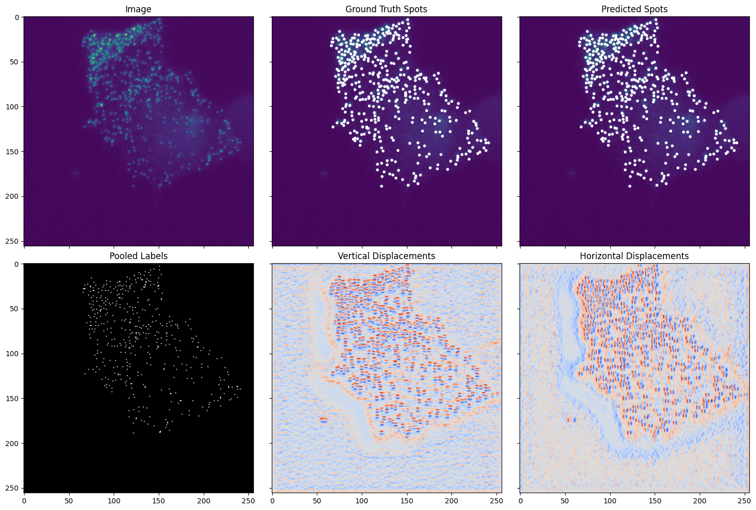
The visualizations compare the Piscis model’s predictions to the ground truth. The input image (top left) contains fluorescent spots targeted for inference. Ground truth spots (top middle) are overlaid as white dots. Predicted spots (top right) are similarly overlaid, aligning strongly with the ground truth. Intermediate feature maps (bottom) are the raw model outputs that are post-processed to generate the final predictions.
Model Input#
Piscis expects the input to be a numpy array. The .predict method offers flexibility in handling various input dimensions to accommodate different imaging datasets. Below are the supported input formats and required parameters for .predict:
- Single Image, 2D (Y, X):
Set the
stackparameter toFalse.Example use case: Predicting on a single-plane image.
- Single Image, 3D (Z, Y, X):
Set the
stackparameter toTrue.Example use case: Predicting on a Z-stack.
- Batch of Images, 2D (Batch, Y, X):
Set the
stackparameter toFalse.Example use case: Predicting on a batch of independent single-plane images (this is the case in the above guide).
- Batch of Images, 3D (Batch, Z, Y, X):
Set the
stackparameter toTrue.Example use case: Predicting on a batch of independent Z-stacks.
Piscis also supports models trained on multi-channel images, where the input includes a channel axis. In general, the axes order for inputs is (Batch, Z, C, Y, X), where:
Batch: Number of images in the batch.
Z: Number of slices in Z.
C: Number of channels (only included if the model was trained on multi-channel images).
Y, X: Spatial dimensions.
Note: All pre-trained models, including 20251212, accept only single-channel inputs. In this case, the channel dimension is omitted from the input. If you train a custom model on multi-channel images, ensure the axes are ordered correctly and adjust the stack parameter accordingly.